|
NPSpec
0.2.0
Solve for the spectral properties of nanoparticles easily
|
|
NPSpec
0.2.0
Solve for the spectral properties of nanoparticles easily
|
NPSpec calculates the spectral properties of the nanoparticle by determining the frequncy-dependent polarizability, from which its optical properties can be calculated. The polarizabiliy is calculated using one of two formulas: Mie theory[6][2] to simulate spheres, and the quasistatic approximation to simulate spheroids.[2] Mie theory is an analytical solution to Maxwell's equations for spheres; Mie theory will not be derived here, but the reader is directed to Chapter 4 of Ref.[2] for an in-depth presentation. The Mie theory code used is based on n-mie which is available for free online.[8] n-mie is capable of calculating the optical efficiencies for an \(n\)-layered sphere, but NPSpec limits this to a 10 layered core@shell particle for practical reasons.
The quasistatic approxomation for spheroids is described in detail in Chapter 5 of Ref.[2], and will be summarized here. To use the quasistatic approximation, the nanoparticle volume \(V\), dielectric constant \(\epsilon(\omega)\), and geometrical factor \(g_{\alpha,d}\) must be known; if these are known, the frequency-dependent polarizability of the nanoparticle in a vacuum is
\[ \alpha_{\alpha\alpha}(\omega) = V \frac{\epsilon(\omega) - 1 }{ 1 + g_{\alpha,d} (\epsilon(\omega) - 1)} \]
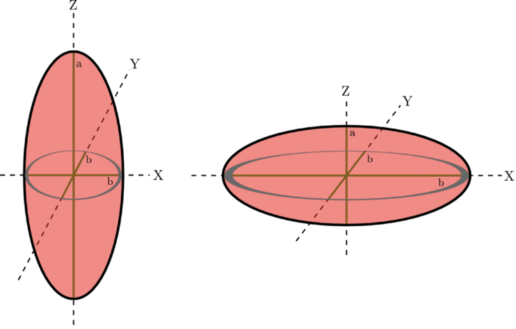
where the diagonal polarizability component that is solved for is based on the direction of \(g_{\alpha,d}\). In NPSpec, the shape of the nanoparticle is limited to spheroids because these shapes have analytical forms for \(g_{\alpha,d}\). Spheroids are defined to have one independent axis \(a\) and two dependent axes \(b\) as shown in the figure above; if \(a\) is longer than \(b\), the spheroid is prolate (cigar-shaped), but if \(a\) is shorter than \(b\) it is oblate (pancake-shaped). If \(a=b\), it is a sphere. The subscript \(d\) in \(g_{\alpha,d}\) indicates the axis component ( \(a\) or \(b\)) of the spheroid. The volume of the nanoparticle is given by
\[ V = \frac{4\pi}{3}ab^2 \ . \]
In the case of a sphere, the geometry factor is[2]
\[ g_{\alpha,d}^\text{sphere} = \frac{1}{3} \ . \]
For a prolate spheroid,
\begin{gather} g_{\alpha,a}^\text{prolate} = \frac{1-e^2}{e^2}\left(-1 + \frac{1}{2e}\ln\frac{1 + e}{1 - e}\right) \\ g_{\alpha,b}^\text{prolate} = \frac{1-g_{\alpha,a}^\text{prolate}}{2} \end{gather}
where
\[ e = 1 - \frac{b^2}{a^2} \ . \]
For an oblate spheroid,
\begin{gather} g_{\alpha,b}^\text{oblate} = \frac{h(e)}{2e^2}\left[\frac{\pi}{2} - \tan^{-1}h(e)\right] - \frac{h^2(e)}{2} \\ g_{\alpha,a}^\text{oblate} = 1 - 2g_{\alpha,b}^\text{oblate} \end{gather}
where
\begin{gather*} h(e) = \sqrt{\frac{1 - e^2}{e^2}} \\ e^2 = 1 - \frac{a^2}{b^2} \ . \end{gather*}
The above formula for the polarizability can be extended to calculate a nanoparticle in a dielectric medium as
\[ \alpha_{\alpha\alpha}(\omega) = V \frac{\epsilon(\omega) - \epsilon_m } { \epsilon_m + g_{\alpha,d} (\epsilon(\omega) - \epsilon_m)} \label{seecoseq:quasi} \]
where \(\epsilon_m\) is the dielectric of the medium (the solvent). Additionally, because NPSpec allows for the calculation of a core@shell nanoparticle, an extended form of the above equation that allows for a two layered particle is necessary and is given by
\[ \alpha_{\alpha\alpha}(\omega) = V \frac{(\epsilon_\text{shell}(\omega) - \epsilon_m) (\epsilon_\text{shell}(\omega) + ab) + af\epsilon_\text{shell} } {(\epsilon_\text{shell}(\omega) + ab) (\epsilon_m + g_{\alpha,d}^\text{shell}(\epsilon_\text{shell}(\omega) - \epsilon_m)) + afg_{\alpha,d}^\text{shell}\epsilon_\text{shell} } \]
where \(a = \epsilon_\text{core}(\omega) - \epsilon_\text{shell}(\omega)\), \(b = g_{\alpha,d}^\text{core} - fg_{\alpha,d}^\text{shell}\), and \(f\) is the fraction of the total nanoparticle volume of the core.
The formula for the absorption, scattering, and extinction efficiencies within the quasistatic approximation are given by
\begin{gather} q^\text{abs}(\omega) = \frac{x}{\pi R^3}\Im\{\bar{\mathbf{\alpha}}\} \\ q^\text{scat}(\omega) = \frac{x^4}{6\pi^2 R^6}\left|\bar{\mathbf{\alpha}}\right|^2 \\ q^\text{ext}(\omega) = q^\text{abs}(\omega) + q^\text{scat}(\omega) \end{gather}
where \(x = 2\pi n_mR/\lambda\) is the size parameter, \(n_m\) is the refractive index of the medium, \(\lambda\) is the wavelength of the incident light, \(R\) is the nanoparticle radius, and \(\Im\{\bar{\mathbf{\alpha}}\}\) is the imaginary component of the isotropic polarizability. For spheroids, we use the radius of a sphere with the same volume as the spheroid for \(R\). Because spheroids are calculated within the quasistatic approximation, it is necessary to limit the size of the spheroid. By comparing the absorption and scattering efficiencies calculated with Mie theory against those calculated with the quasistatic approximation for a sphere, we find that an upper limit for the size parameter of 3 is acceptable; this corresponds to an effective \(R\) of about 15 nm.
All dielectric constants are taken from the handbook of Palik.[9] They have been pre-splined and hard-coded into the NPSpec library for wavelengths from 200-999 nm (inclusive) in increments of 1 nm. A select few materials also have size-correction parameters implemented, which may be useful for nanoparticles with a radius < 3 nm. Briefly, the free electrons in smaller nanoparticles have a longer mean free path than the size of the nanoparticle so the electrons scatter off the surface; this causes the spectrum to broaden. To perform a size correction requires knowing the drude function for the free electrons of the nanoparticle material and the fermi velocity of the electrons in the nanoparticle material. The drude function is given by[2]
\[ \epsilon(\omega)_\text{drude} = \epsilon_{\infty} - \frac{\omega_p^2}{\omega^2+i\gamma\omega} \]
where \(\epsilon_{\infty}\) is the dielectric at infinite frequency, \(\omega_p\) is the free electron plasma frequency, \(\gamma\) is the free electron excited state decay rate. The size correction parameter is given by
\[ s = \frac{v\hbar}{R} \]
where \(v\) is the fermi velocity and \(R\) is the nanoparticle radius. To perform the size correction, the uncorrected drude function is subtracted from the experimental dielectric function, and then the size-corrected drude function is then added back in:
\[ \epsilon(\omega)_\text{corrected} = \epsilon(\omega) + \frac{\omega_p^2}{\omega^2+i\gamma\omega} - \frac{\omega_p^2}{\omega^2+i(\gamma+s)\omega} \]
The drude functions and fermi velocities were taken from several sources. [10][1][5][4]
The colors are predicted from the absorption or scattering efficiency spectrum by converting the spectrum into RBG colors values using the International Commission on Illumination (CIE) 1931 color system and D65 daylight illuminant.[11][3] For absorbance, the spectrum is converted first to transmission using
\[ \text{TRAN} = 10^{-q^\text{abs}} \]
and for scattering the spectrum is simply normalized.
 1.8.3.1

